1. Introduction

Figure 1: The figure show three lines separating the black and the green group.

This blog post is about Support Vector Machines (SVM), but not only about SVMs. SVMs belong to the class of classification algorithms and are used to separate one or more groups. In it’s pure form an SVM is a linear separator, meaning that SVMs can only separate groups using a a straight line. However ANY linear classifier can be transformed to a nonlinear classifier and SVMs are excellent to explain how this can be done. For a deeper introduction to the topic I recommend Tibshirani (2009), one can find a more detailed description including an derivation of the complete lagrangian there.

The general Idea of SVM is to separate two (or more) groups using a straight line (see Figure 1). However, in general there exits infinitely many lines that fulfill the task. So which one is the “correct” one? The SVM answers this question by choosing the line (or hyperplane if we suppose more than two features) which is most far away (the distance is denoted by $\zeta$ ) from the nearest points within each group.

2. Mathematical Formulation

2.1 Separating Hyperplanes

Suppose multivariate data given by a pair where the explanatory variable $x \in \mathbb{R}^p$ and the group coding $y \in {-1,1}$ . In the following we assume an iid. sample of size given by $(y_1,x_1),\dots,(y_N,x_N)$ .\
Any separating hyperplane (which is a line if ) can therefore be described such that there exits some $\beta\in \mathbb{R}^p$ and

(1) $\begin{equation*} y_i(x_i^T \beta + \beta_0) \geq \zeta >0, \; \forall i=1,\dots,N. \end{equation*}$

Note that with the (non restrictive) condition that $||\beta||=1$ . Our task to separate the groups is covered by the minimization problem

(2) $\begin{equation*} min_{\beta,\beta_0} ||\beta|| \; s.t. \; y_i(x_i^T \beta + \beta_0) >1, \; i=1,\dots,N. \end{equation*}$

2.2 Support Vector Machines

In most cases the assumption that there exits a hyperplane that perfectly parts the data points is unrealistic. Usually some points will lie on the other side of the hyperplane. In that case (2) will not have a solution. The idea of SVM is now to introduce an parameter $\xi$ to fix this issue. In particular we modify (1) such that we require\

(3) $\begin{equation*} y_i(x_i^T \beta + \beta_0) \geq \zeta(1 -\xi_i), \; \forall i \, \xi_i >0, \; \sum_{i=1}^N \xi_i < \infty. \end{equation*}$

The corresponding minimization problem is then given by

(4) $\begin{equation*} min_{\beta,\beta_0} ||\beta|| \; s.t. \; y_i(x_i^T \beta + \beta_0) > 1 -\xi_i,\xi_i \geq 0 \; \forall i, \; \sum \xi_i \leq C < \infty \end{equation*}$

Both (2) and (3) are convex optimization problems and can be solved for example using the Lagrange minimization technique. A solution for (4) always has the form

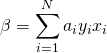
(5) $\begin{equation*} \beta=\sum_{i=1}^N a_i y_i x_i \end{equation*}$

where iff (3) is met with “” and else, these are then called support vectors.

2.2 Nonlinear SVMs

Figure 2: The figure shows an example of two groups which are not separating using a straight line.

The method we described so far can only handle data where the groups can be separate using some hyperplane (line). However in many cases the data to be considered is not suited to be separated using a linear method. See figure 2 for example, in figure 2 the groups are arranged in two circles with different radius. Any attempt to separate the groups using a line will thus fail. However any linear method can be transformed into a non-linear method by projecting the data into a higher dimensional space. This new data $\phi(x)$ may then be separable by some linear method. In case of figure 2 a suitable projection is for example given by $\phi(x)=(x_1,x_2, x_1^2 + x^2)$ , $\phi(x)$ maps the data onto a cone where the data can be separated using a hyperplane as to be seen in figure 3. However, there are some drawbacks using this method. First of all $\phi$ will in general be unknown. In our simple example we where lucky to find a suitable $\phi$ , however concerning a more complicated data structure fining a suitable $\phi$ turns out to be very hard. Secondly, depending on the dataset, the dimension of $\phi$ needed to guarantee the existence of a separating hyperplane can become quite large and even infinite. Before we deal with this issues using kernels we will first have a look at the modified minimization problem (4) using $\phi(x)$ instead of .

Let the nonlinear solution function given by $f(x)= \phi(x)^T \beta+\beta_0$ . To overcome the need of the constant we introduce some penalty $\lambda>0$ and rewrite (4) as\

(6) $\begin{equation*} min_{\beta_0,\beta} \sum_{i=1}^N [1- y_i f(x_i)]_+ \frac{\lambda}{2} ||\beta||^2. \end{equation*}$

\
The notation means that only the positive part of is taken into account.
At this point I would like to establish the connection to other linear methods. Since we consider SVMs we set the Loss function to . Different loss functions will lead to different methods, for example using will correspond to the logistic regression. Therefore the following strategy can be used to extent linear methods to deliver non-linear solutions.

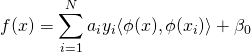
From (5) we already know, that a nonlinear solution function will have the form\

(7) $\begin{equation*} f(x)=\sum_{i=1}^N a_i y_i \langle\phi(x),\phi(x_i)\rangle +\beta_0 \end{equation*}$

\
We can verify, that knowledge about $\phi$ is in fact not required to formulate the solution. We only need to know something about the inner product $\langle\phi(x),\phi(x_i)\rangle$ . While $\phi(x)$ could be a high dimensional complicated function, the inner product is just a number. So if we would have some magical procedure that gives us this number, solving Nonlinear SVM would be straightforward. This leads us to think about kernels.

2.2.1 Kernels

Figure 3: The same example as above. Projection to a space using one addition dimension makes the groups again separable using a hyperplane.

We already get in touch with kernels when estimating densities or a regression. In this application Kernels are a way to reduce the infinite-dimensional problem to a finite dimensional optimization problem because the complexity of the optimization problem remains only dependent on the dimensionality of the input space and not of the feature space. To see this, let $x,z \in \mathbb{R}^p$ instead of looking at some particular function $\phi(x)$ , we consider the whole space of functions generated by the linear span of ${K(·,z), z \in \mathbb{R}^p)}$ where $\phi(x)$ is just one element in this space. To model this space in practice popular kernels are

linear kernel: $K(x,z)=\langle x,z\rangle$
polynomial kernel: $K(x,z)=\langle x,z\rangle ^{{d}}$
radial kernel: $K(x,z)=\exp \left(-{\tfrac {||x-z||^{{2}}}{2\sigma ^{{2}}}}\right)$

used. Choosing a kernel that naturally fits the structure of the date is beneficial. In our example from figure 2, the radial kernel is a good choice.
Suppose that has an eigen-expansion

(8) $\begin{equation*} K(x, z)= \sum_{j=1}^\infty \gamma_j \varphi_j(z) \varphi_j(x) \end{equation*}$

where $\varphi$ are the orthonormal eigenfunctions of and eigenvalues $\gamma_i\geq 0$ , $\sum \gamma_i^2 < \infty$ which ensure that that the generated space is a Hilbert space. Then $\phi(x)= \sum_{j=1}^\infty \delta_j \varphi_j(x)$ for suitable $\delta$ and for some $c_j=\sum_{i=1}^N \alpha_i \gamma_j \varphi_j(x_i) ,j=1,\dots,\infty$ we can represent

(9) $\begin{equation*} f(x) = \sum_{j=1}^\infty c_j \varphi_j(x) =\sum_{i=1}^N \alpha_i K(x,x_i). \end{equation*}$

\
Thus we can write (6) in its general form as\

(10) $\begin{equation*} min_c_j \sum_{i=1}^N L(y_i, \sum_{j=1}^\infty c_j \varphi_j(x_i)) + \lambda \sum_{j=1}^\infty c_j^2/\gamma_j \end{equation*}$

\
According to (9) we can write down (10) using matrix notation $\mathbf{K}_{ij} = K(x_i,x_j),\;i,j=1,\dots,N \; \mathbf{y}=(y_1,\dots,y_N),\; \mathbf{\alpha}=(\alpha_1,\dots,\alpha_N)$ as

(11) $\begin{equation*} min_\mathbf{\alpha} L(\mathbf{y}, \mathbf{K} \mathbf{\alpha}) + \lambda \mathbf{\alpha}^T \mathbf{K} \mathbf{\alpha}. \end{equation*}$

This finite dimensional problem can now be solved using standard methods.

1,706

Non-Linear Support Vector Machines (SVM)